eSports — a form of sports where the primary aspects are facilitated by electronic systems — provide unique opportunities to mine and analyze data. Every aspect of eSports matches can be recorded digitally and analyzed with software, vastly reducing the energy required to collect and interpret patterns. The recent MLG Major Counter-Strike Global Offensive competition in Columbus, Ohio is one of these opportunities.
Counter-Strike: Global Offensive (CS:GO) is an internationally acclaimed competitive skill-based First Person Shooter developed by Valve LLC. Released in 2000, it has a long history in competitive gaming (eSports), attracting over a million viewers at the 2016 Major League Gaming competition in Columbus, Ohio.
In competitive mode, matches are broken down as follows:
Originally, this project’s aim was to ascertain the impact winning a pistol round in Counter-Strike: Global Offensive has on winning the match. As the data grew, the scope of this project increased beyond this single question to a general analysis of the effectiveness of teams’ economic management.
HLTV.org keeps a brilliant searchable index of historical CS:GO matches. To focus on the Columbus 2016 competition, set Events to MLG Columbus 2016 and download the demo files for each match. Demo files contain highly compressed information about matches. They allow users to accurately recreate matches inside the game engine. Demo files also provide a unique window for analyzing play without manually recording a single piece of data.
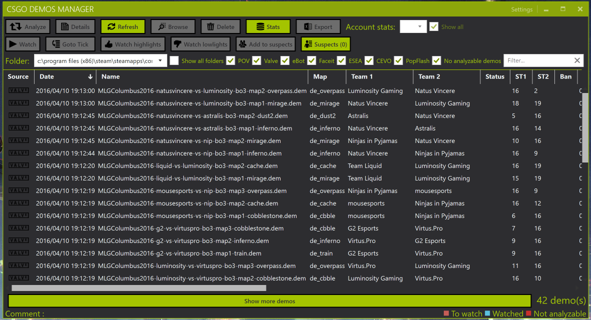
CSGO-Demos-Manager is an invaluable open-source tool for analyzing CS:GO demo files. It will “play” through a demo, tracking many different variables. Because the project is open source, it is easily extensible. However, it only runs on Windows.
Once CSGO-Demos-Manager has analyzed the relevant demo files, users can choose to export the data to Excel as a group or individually. Both of the exports look more or less the same: a 6-sheet Excel table:
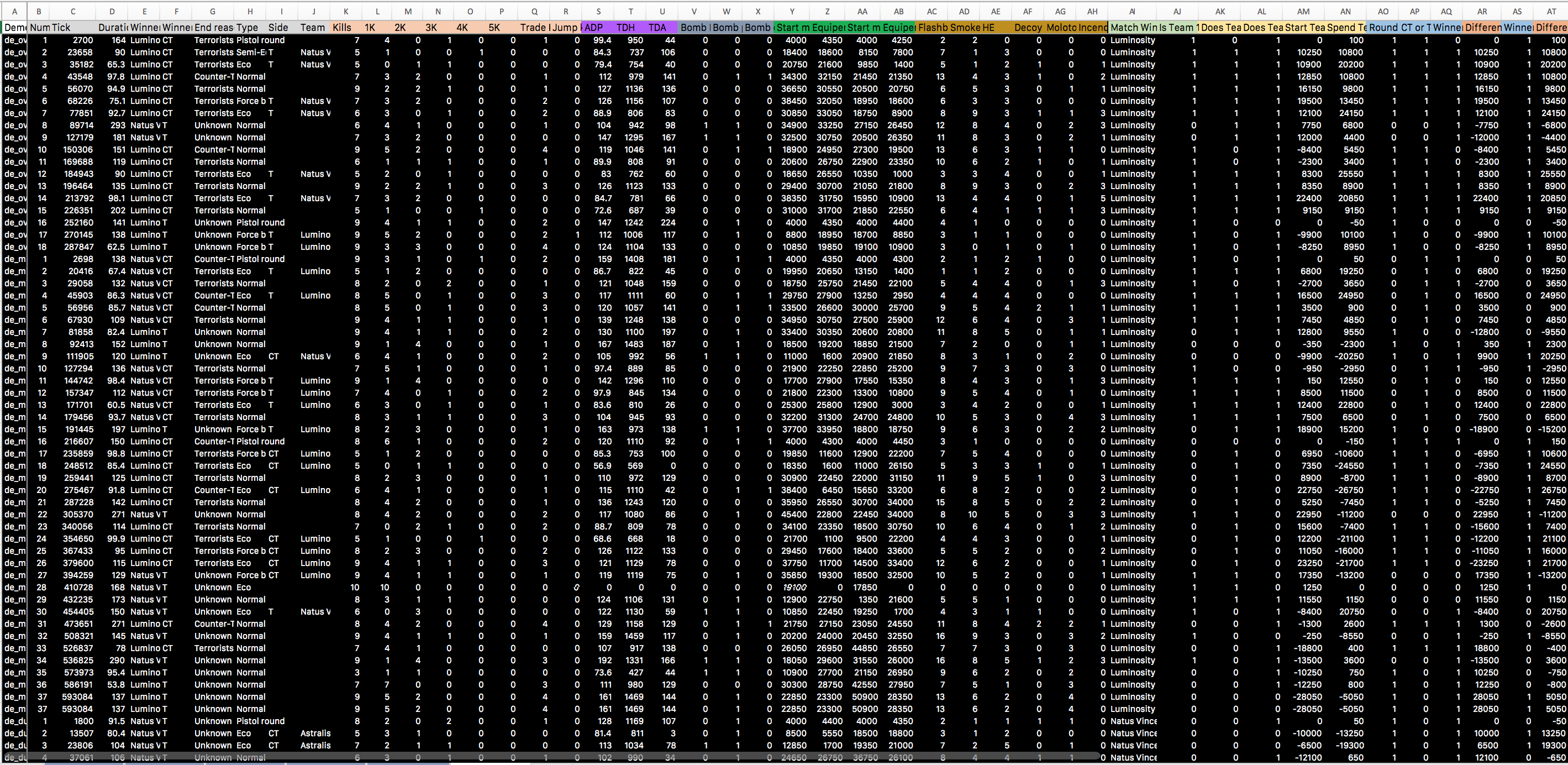
This provides a strong basis to start analyzing various aspects of the event as well as ascertain important levels of performance.
The most important column to add to the table is also the most tedious. Before the CSGO-Demos-Manager created column Number1 it is best to a new column, Demo ID. This creates a faux primary key2 to compare individual matches with ending match results. Without this, there is no way to pull data related to the overall match from the General sheet to the Rounds sheet. To do this, manually copy the relevant Demo ID from column B on the General sheet.
Sadly, CSGO-Demos-Manager improperly symbolicates the Winner column. To resolve this, replace that column with the following formula3: =IF(N2>O2,L2,M2).
This checks if Team 1’s score is larger than Team 2’s score. If this case is met, the formula outputs Team 1’s name; if the case is not met, it outputs Team 2’s name.
The Rounds tab can now be related to the General sheet thanks to the Demo ID column added earlier.
This column references the General sheet and tells us what the winner of the entire match is. This is important when looking for variables that affect the outcome of entire matches and not individual rounds. To do this, use =VLOOKUP(A2,General!B:AT,19,FALSE).4
As a sanity check, the Match Winner column should remain the same for a given set of rounds. It does, so this calculation appears accurate.
Now that the data shows who won the overall match, it is trivial to see how often a match winner was a round winner. The simple formula =IF(AJ2=E2,1,0) checks if the winner of the round is the same as the winner of the match. It returns a dummy variable, 0, if the teams do not match and 1 if they do.
As a sanity check, this column should have a larger sum than the number of rows since winners naturally have more round wins. The spreadsheet has 1,112 rows, 663 of which read 1, so this calculation appears accurate.
Now that the data has been adequately prepared, the real work can begin. Both Excel and Stata prove to be integral tools for analyzing and visualizing the data sets.
For simpler analysis and visualization, Excel’s tools are easy to use and works well.
The original research question posited that the pistol round positively influenced a team’s chance to win the match. This is easily ascertained with a basic Excel analysis.
First, the relevant data must be extracted from the Rounds sheet. We can use the Match Winner column created earlier to make a simple dummy variable to simplify counting. Insert a new column to the right of the dataset called Round Winner = Match Winner? and use =IF(AI2=E2,1,0) to check if the Match Winner is the same as the Round Winner. If they are the same, the equation returns 1. If not it returns 0.5
Once the Round Winner = Match Winner? column has been created, it is simple to count the data with a simple =COUNTIF formula. Create two cells far off to the right of the data and use the following formula: =COUNTIFS(H:H,"Pistol round", AO:AO,1). This checks the Type column and restricts it to pistol rounds and then counts the frequency of 1 in the Round Winner = Match Winner? column. Directly this we use `=COUNTIFS(H:H,"Pistol round", AO:AO,0) to get the frequency of 0 in the same column.
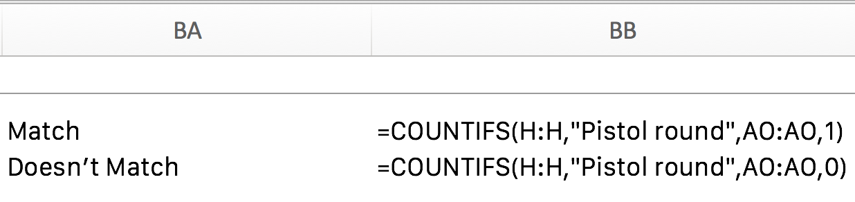
Simple division with =BB2/COUNTIF(H:H, "Pistol round") and =BB3/COUNTIF(H:H, "Pistol round”) allow us to calculate the proportion of wins and losses. According to the data, this results in:
| Type | Value | Proportion |
|---|---|---|
| Match | 55 | 67% |
| Doesn’t Match | 27 | 33% |
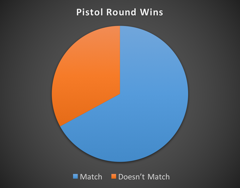
The data shows a 67% match rate, which indicates that the Pistol Round winner is the Match Winner 67% of the time. This is to say that winning the pistol round achieves a 2/3 probability of winning the entire match. To clarify, the word “Match” in the chart indicates rounds where the pistol round winner matches the match winner.
Before calculating the impact resources has on a match, the data must describe the frequency of economic impact on individual rounds. This can partially be calculated in Excel, however more advanced analysis will require Stata.
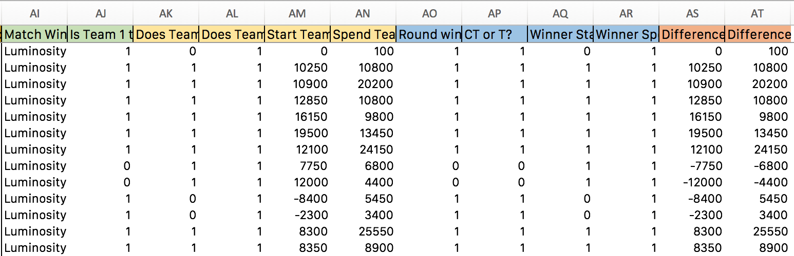
First, it is necessary to create a new formula that outputs a dummy variable. 1 should define when the winner has more resources, 0 should define when the winner has less. The simplest way to accomplish this is to create a new column called Winner Spend More On Equipment? and reference the General sheet and Match Winner column:
=IF(IF(Z2>AB2,VLOOKUP(A2,General!B:AT,11,FALSE),VLOOKUP(A2,General!B:AT,12,FALSE))=AI2,1,0)This formula uses a nested =IF. The interior statement checks if Team 1 starts with more equipment than Team 2. If Team one starts with more, the formula pulls Team 1’s name from the General sheet. If Team 2 starts with more, it pulls that name instead. Next, the exterior statement compares the string result from the interior statement to the string in the Match Winner column. If the strings match, Team 1 is the winner, and the formula outputs a 1. If Team 2 is the winner, the formula outputs 0. This column now calculates which team has better equipment and if having better equipment corresponds with a win.
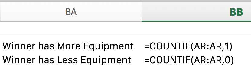
As before, use =COUNTIF(AR:AR,1) and =COUNTIF(AR:AR,0) to count the frequency at which this specific test occurs. This formula is far simpler than before because we are not using other columns to restrict counting.
| Type | Value | Proportion |
|---|---|---|
| Winner has More Equipment | 633 | 60% |
| Winner has Less Equipment | 449 | 40% |
Further, =BB8/SUM(BB8:BB9) and =BB9/SUM(BB8:BB9) can be used to calculate the relevant proportion.
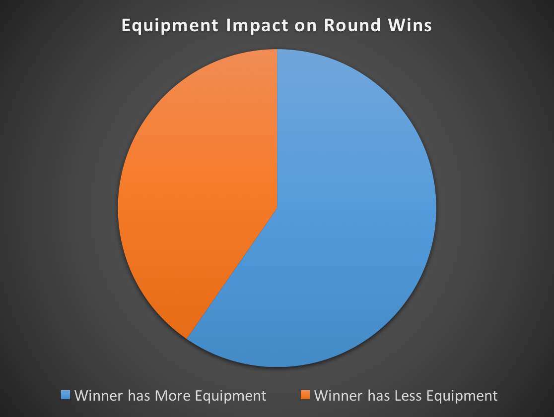
The winner has better equipment 60% of the time — barely more than half. This demonstrates that, at the professional level, the game’s economy has little effect on various outcomes.
Sadly, Excel hits a wall when it comes to more advanced econometric plotting and analysis. However, Stata’s data entry system can be slow and arduous; it is often a better choice to use Excel to create the data and then simply copy it into Stata. This section will describe several new columns that will not be used in the Excel analysis but will come into play for the Stata section.
These columns in the Rounds sheet are as follows:
=VLOOKUP(A2,General!B:AT,19,FALSE)general sheet.=IF(VLOOKUP(A2,General!B:AT,11,FALSE)=E2,1,0)=IF(Y2>AA2,1,0)=IF(Z2>AB2,1,0)=Y2-AA2=Z2-AB2=IF(AI2=E2,1,0)=IF(F2="CT",1,0)=IF to create a dummy variable 1 if the Winner starts with more money and 0 if notwinner spend more on equipment outlined above=IF(IF(Y2>AA2,VLOOKUP(A2,General!B:AT,11,FALSE),VLOOKUP(A2,General!B:AT,12,FALSE))=AI2,1,0)=IF(IF(Z2>AB2,VLOOKUP(A2,General!B:AT,11,FALSE),VLOOKUP(A2,General!B:AT,12,FALSE))=AI2,1,0)=IF(VLOOKUP(A2,General!B:AT,11,FALSE)=E2,Y2-AA2,AA2-Y2)=IF(VLOOKUP(A2,General!B:AT,11,FALSE)=E2,Z2-AB2,AB2-Z2)State provides a robust platform for advanced econometric analysis.
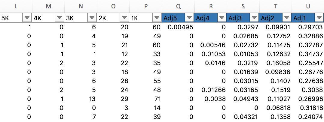
The first visualization in Stata is relatively simple. First, we must adjust the kill data on the Players sheet of MLG2016Full.xlsx. This adjustment will account for the amount of rounds players participated in. If the data is not adjusted, players that played more rounds that have higher overall totals will end up above players that have a higher ratio of kills per round.
To accomplish this, add 5 columns, one for each kill quantity.9 Because the number of rounds played is static, the formula =L2/$J2 can be used to calculate the correct ratios. Locking the denominator to the J column ensures the Rounds column is always used while also allowing the formula to be filled relatively.
Next, the kill totals must also be adjusted. Adding a column next to kills with =D2/C210 will adjust the kill count to a per-match ratio. If we do not adjust the kill totals, we get skewed output like this:
The file MLGPlayerData.dta attached below already has these columns inserted.
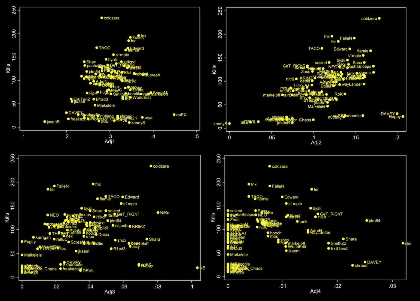
Once the data is imported to Stata, we use the scatter command to make the scatterplot. To scatter Total Kills to the Adjusted 1K Ratio, enter scatter killspermatch adj1, mlabel(name). To scatter the other adjusted kill ratios, use adj2, adj3, and so on. Adding ,mlabel(name) tags each point with the corresponding player name.
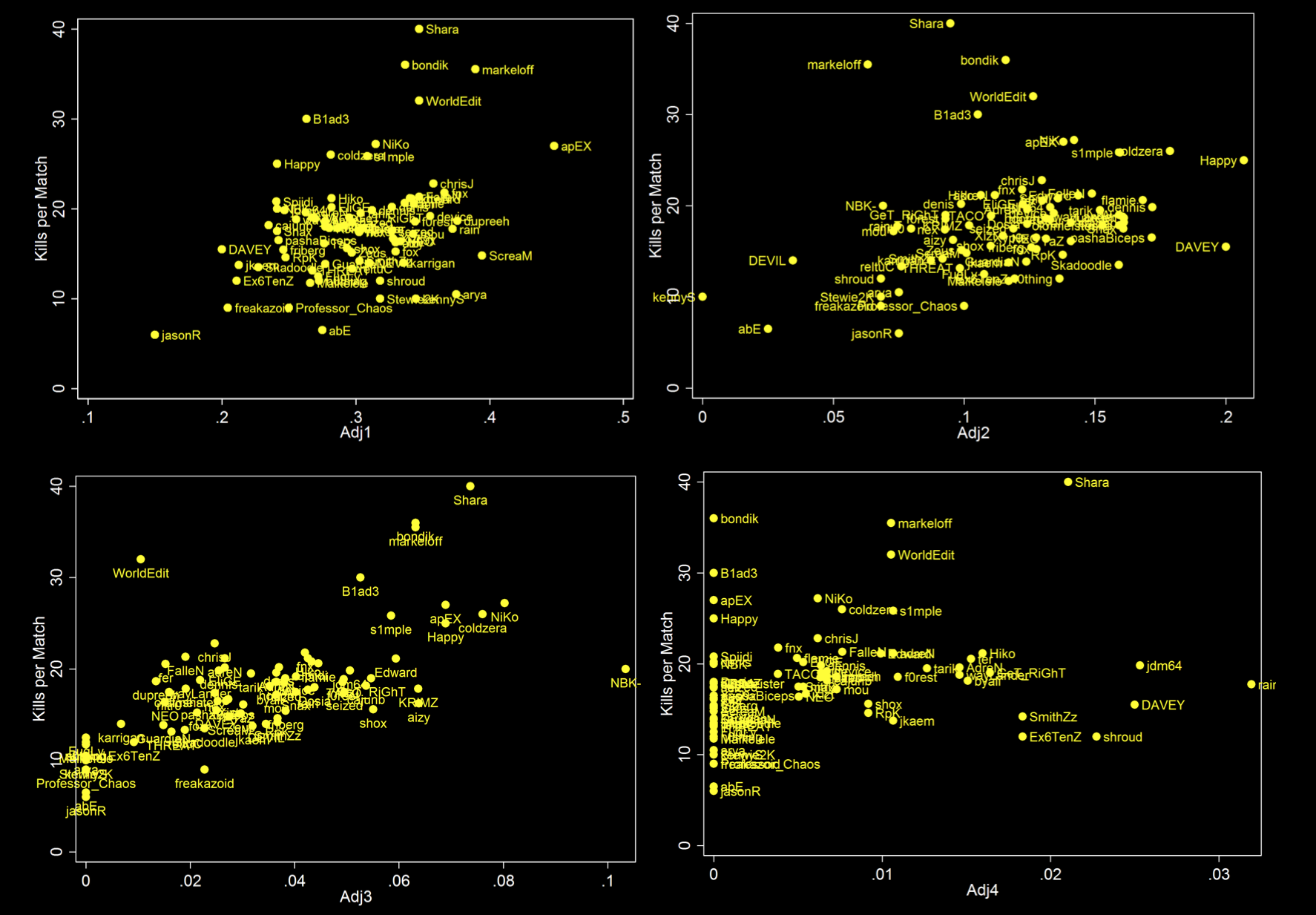
Vertical height denotes more overall kills per round. Horizontal extension denotes the propensity of a player to hit that certain amount of kills: the further right a player is, the more often they hit that number of kills per round.
I omitted adj5 from this visualization because only 7 players achieved 5k.11 There is not enough data to draw a reasonable conclusion.
Each round rewards players with various income based on individual and group performance. Regression models can describe how the gameplay economy affects match outcomes.
The Rounds sheet holds all of the data used for the regression analysis. Thanks to the columns added prior, copying and pasting directly into Stata allows us to dove right into the data.12
These imported variable names are quite long. Luckily, Stata has an autocomplete feature: press the Tab key to bring up a list of variables that complete the text entered in the command line.
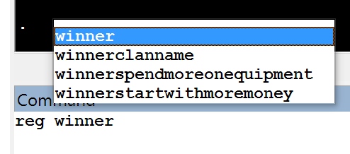
Regressing variables onto isteam1thewinner will find the impact said variables have on influencing Team 1 to beat Team 2. For example, reg isteam1thewinner equipementvalueteam1 equipementvalueteam2 does a multiple regression to ascertain the effects variables equipementvalueteam1 and equipementvalueteam2 have on the variable isteam1thewinner. This command results in:
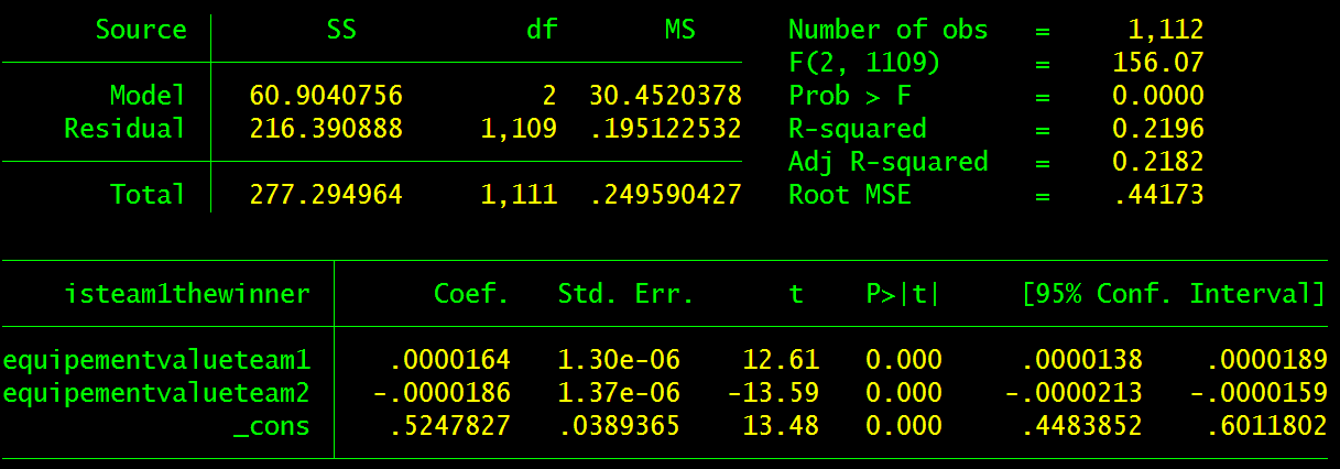
This tells is that β2 and β3 — the respecive effects of equipementvalueteam1 and equipementvalueteam2 — have inverse impacts on Team 1 winning a round (y). β1, the constant, shows that if both teams are equal, there is a 50% chance that team 1 wins.
The full equation reads y = 0.0000164x - 0.0000186z + 52.5 where x is the dollar value of Team 1’s gear and z is the dollar value of Team 2’s gear. Each dollar of Team 1 gear raises their chance of winning by 0.00164% and each dollar of Team 2 Gear lowers Team 1’s chance of winning by 0.00186%. All things considered, this results in very little economic impact on professional gameplay unless there are large differences in the buying power of each team.
The variable doesteam1havemoreequipment allows us to perform another simple regression onto isteam1thewinner, this time to determine the overall effect of having more equipment.
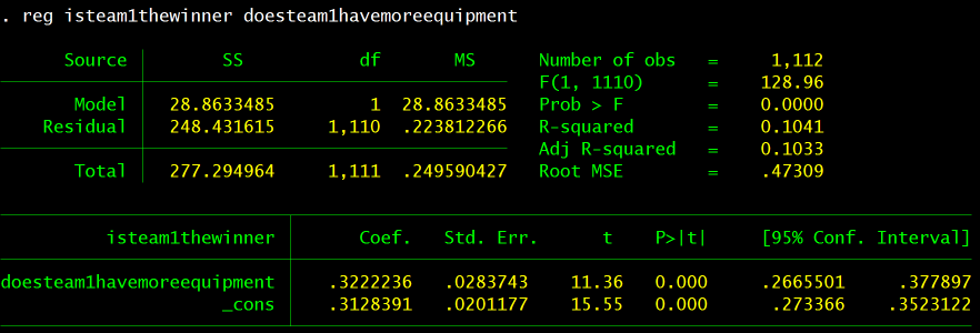
The constant here is approximately 0.31 while β2 is about 0.32. This means the regression line would be y=0.32x + 0.31 where y is the percent chance of winning. This tells us that there is a 31% chance of winning when Team 1 has less equipment and a 63% chance of winning when Team 1 has more equipment. This confirms the earlier Excel analysis that posited the winner has more equipment 60% of the time:
| Type | Value | Proportion |
|---|---|---|
| Winner has More Equipment | 633 | 60% |
| Winner has Less Equipment | 449 | 40% |
Value of team inventories occasionally forces teams to save and purposely not buy inventory — a strategy dubbed Eco or Semi-eco to try and push back later. CSGO-Demos-Manager is able to automatically analyze the type of round and conveniently creates a Type column that contains the information:
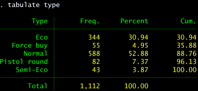
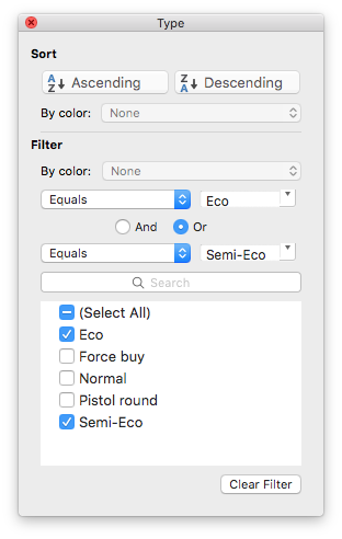
To study the effects of this strategy the data needs to be restricted to only show Eco and Semi-eco rounds: simply filter the Type column on the Round sheet.13
Once the data has been restricted and imported to Stata, regressing doesteam1havemoremoney onto isteam1thewinner elucidates the effects of better equipment:
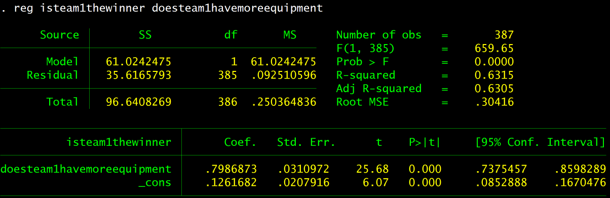
The regression line is y = 0.79x + 0.126. This tells us that having more equipment — β2 — raises the odds of winning an eco or semi-eco round by 79%. While this is high, it means that variables other than equipment affect the outcome of eco rounds – but only 9% of the time.
This data comes in 3 major formats: Demo (.dem), Excel (.xlsx), and Stata (.dta). HLTV.org hosts the demo files. All of the files used are located in the /data directory of this post. These are the individual files with respective descriptions:
General contains a summary for each match
Winner column augmented with formula =IF(N2>O2,L2,M2)Players contains statistics for each player
K/D column augmented with formula =D2/F2Maps contains map statisticsTeams contains team statisticsWeapons contains various weapon statistics
Damage per Shot calculated with =D2/E2Damage per Hit calculated with =C2/F2Rounds contains round statistics
Teams sheet of MLG2016Full.xlsxPlayers sheet of MLG2016Full.xlsxRounds sheet of MLG2016Full.xlsxDiscussion on r/GlobalOffensive | View as: PDF / Markdown
Originally “A” ↩︎
Although it is not technically unique, this value serves to relate separate pieces of the data. ↩︎
This assumes you have not modified the existing order of the columns. If you have, use an =IF formula to check if Team 1’s score is larger than Team 2’s score. If true, output Team 1’s name; if false, output Team 2’s name. ↩︎
Again, if you have moved cells around, you will need to use different references. ↩︎
One could also accomplish this without creating a new column by using =COUNTIFS or =SUMIFS and focussing on all three relevant columns, however because later analysis uses the round winner = match winner? column it makes sense to create it now. ↩︎
Actually “Equipment Value” and not “Spend” per se. ↩︎
Actually “Has Better Equipment” and not “Spend More On” per se. ↩︎
Actually “Equipment Values” and not “Spends” per se. ↩︎
Kill quantity refers to how many kills a single player gets in a given round, i.e. 1k is one kill, 2k is 2 kills, 3k is three kills, and so on. ↩︎
Inserting a column here will preserve the references to the right. ↩︎
As a result, everyone is bunched up above the X axis at 0. ↩︎
MLGFull.dta located below contains this data in a pre-made Stata file. ↩︎
Another solution is to use gen or tabulate in Stata, however it is often simpler to adjust the data using Excel filters and create a new Stata file. ↩︎