When you look at the back of a baseball card, you don’t see a single rating. You see time-series information about that player.1 Additionally, they do not use a single number to tell a story about a player. No magic number that will accurately depict a player’s performance. However, with younger sports like Counter-Strike: Global Offensive, the single stat most people focus on is a player’s rating. This single number is problematic for many reasons. With the trove of data we have access to in demo files that we do not have with any other sport, we need to move to something more nuanced.2
Recently, HLTV announced a new rating system for professional CS:GO players. This new system was designed to weight more impactful kills more than less impactful ones. They describe the system as one that “better encapsulates the different ways players contribute in the game.” Statistically speaking this is untrue. HLTV 2.0 provides no statistically discernible difference that improves it in comparison with its predecessor.
According to HLTV, the rating 1.0 system uses three distinct elements:
The formula HLTV uses to calculate the rating can be expressed as follows, where Cs are the respective constants and the summation represents the multi-kill rating:
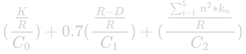
In this context, the Σ calculates an average value for all of the multi-kill events (k1, k2 , etc.) weighted by the square of the number of kills. The constants Cn are overall longitudinal averages:
| Constant (Average) | Symbol | Value |
|---|---|---|
| Kills per Round | C0 | 0.679 |
| Survived Rounds | C1 | 0.317 |
| Multikill Rating | C2 | 1.277 |
This rating system is trivial to calculate in Excel. Since we are given the several constants, leveraging a lookup table allows us to adjust these to determine their respective effects. These Excel formulas calculate the three variables described above.
Since this is simple division, we do not need to use anything complicated to calculate a kill rating:
=(Kills/Rounds)/0.679
This is similarly simple.
=((Rounds-Deaths)/Rounds)/0.317
This is peskier to calculate, but overall contains only simple addition and division.
=((1K+(4*2K)+(9*3K)+(16*4K)+ (25*5K))/Rounds)/1.277
To calculate these all together, simply reference the respective cells and use the Rating 1.0 formula:
=(KillRating+(0.7*SurvivalRating) +MultikillRating)/2.7
These can also all be combined to a single cell:
=(((Kills/Deaths)/0.679)+ (0.7*(((Rounds-Deaths)/Deaths)/0.317))+ (((1K+(4*2K)+(9*3K)+(16*4K)+(25*5K))/Rounds)/1.277))/2.7
Because rating 1.0 relies on simple mathematics and a small cluster of data, it tends to be biased towards rewarding players with higher kill death ratios. This is problematic because kill death ratio is already an entirely useful metric on its own; having two metrics to judge players that tell you the same thing provides no additional insight.
HLTV 1 relies on three constants. This is problematic for several reasons, not the least of which is that they are not the averages anymore.
Primarily, the averages of 0.679, 0.317, and 1.277 are simply wrong. Looking at the averages we see in the actual statistics; these numbers are closer to the following:
| Variable | HLTV Average | Actual Average | Diff |
|---|---|---|---|
| Kills per Round | 0.679 | 0.658 | 0.021 |
| Survived Rounds | 0.317 | 0.318 | 0.001 |
| Multikill Rating | 1.277 | 1.193 | 0.084 |
These averages shift the actual values of rating 1.0. The HLTV 1.0 column uses the original averages, and the Adjusted column uses the actual averages.
| KPR | SPR | MKR | HLTV1 | Adj | Diff |
|---|---|---|---|---|---|
| 0.96 | 0.37 | 2.01 | 1.42 | 1.47 | 0.06 |
| 0.63 | 0.38 | 1.10 | 0.98 | 1.01 | 0.03 |
| 0.51 | 0.36 | 0.66 | 0.77 | 0.79 | 0.02 |
Additionally, static averages do not provide for comparison of individuals. While using a population mean allows you to compare a player against the overall average, it does not enable one to demonstrate how a player performs relative to their mean. This means the average does not account for map differences, team differences, or other variables that account for variances in kills and deaths.
To demonstrate this problem with rating 1.0, we need only run a simple linear regression to determine the effect the kill death ratio has on individual players. Using the Ratio 1.0 table from my database of player statistics, we can confidently say that the kill death ratio explains 88% of the change in rating 1.0:
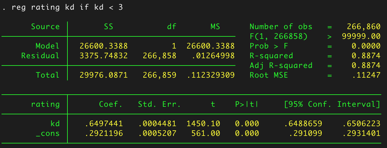
This regression demonstrates that we can use the following formula to estimate rating 1.0 for a player:

This is a far cry from the official equation, yet it nets us 88% of the change. If we instead split the regression into kills and deaths instead of a simple ratio, we get an ever more accurate picture:
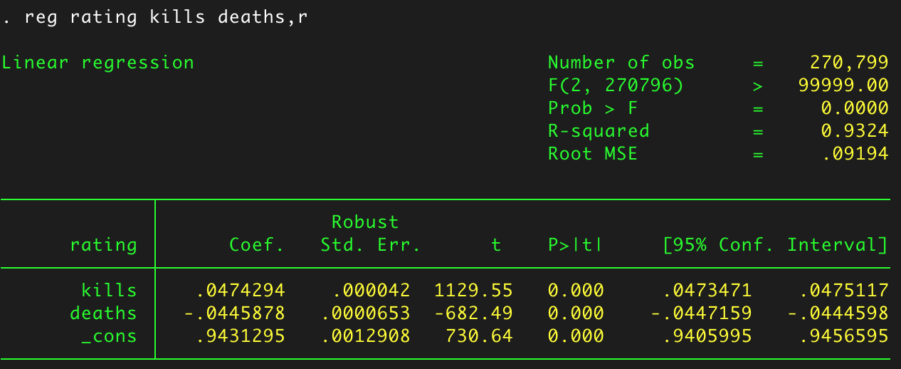
This regression allows us to predict rating 1 with even more accuracy, this time with a 5% improvement in our correlation coefficient. The formula for this regression is as follows:

If we add HLTV’s KAST3 ratio and average damage per round into the mix, the correlation coefficient increases to almost 95%:
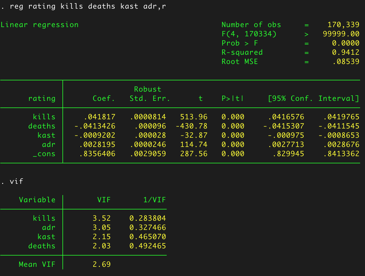
Here, the variance inflation factors demonstrate that there is no multicollinearity problem with the data and that each variable has an effect on the outcome.
Interestingly, here the KAST ratio has a marginally negative effect on a player’s rating: the higher a player’s KAST is, the more negatively it affects a player’s rating.
Using this to predict HLTV Rating 1 and plotting yields this curve:
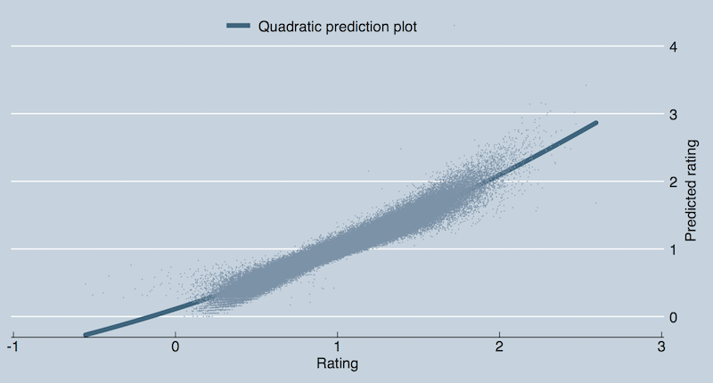
Naturally, there is some degree of error, however explaining over 88% of the change in rating 1 with the kill death ratio is problematic because the entire point of rating 1.0 is to not be a kill death ratio. Because of these problems, HLTV created their rating 2.0 system in June of 2017.
HLTV describes the rating 2.0 system in their blog post:
[Rating 2.0 is] an updated formula for the Rating which we use to quickly assess player performance. It now incorporates data like damage dealt, opening kills, 1onX wins, traded deaths and more, and thus better encapsulates the different ways players contribute in the game.
Graphically, the inputs are interesting to see. This is a more advanced system that incorporates more variables and attempts to explain more variation in player performance.
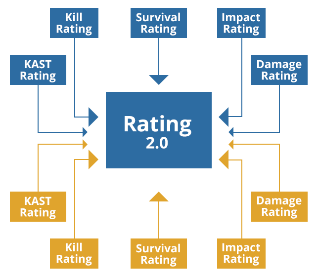
According to the post, it uses ten inputs instead of the previous three (one set of five for each side played):
As they explain, this boosts some players and reduces others. For a sample of the 80 players at PGL Krakow 2017, we can see how Rating 1 and Rating 2 compare:
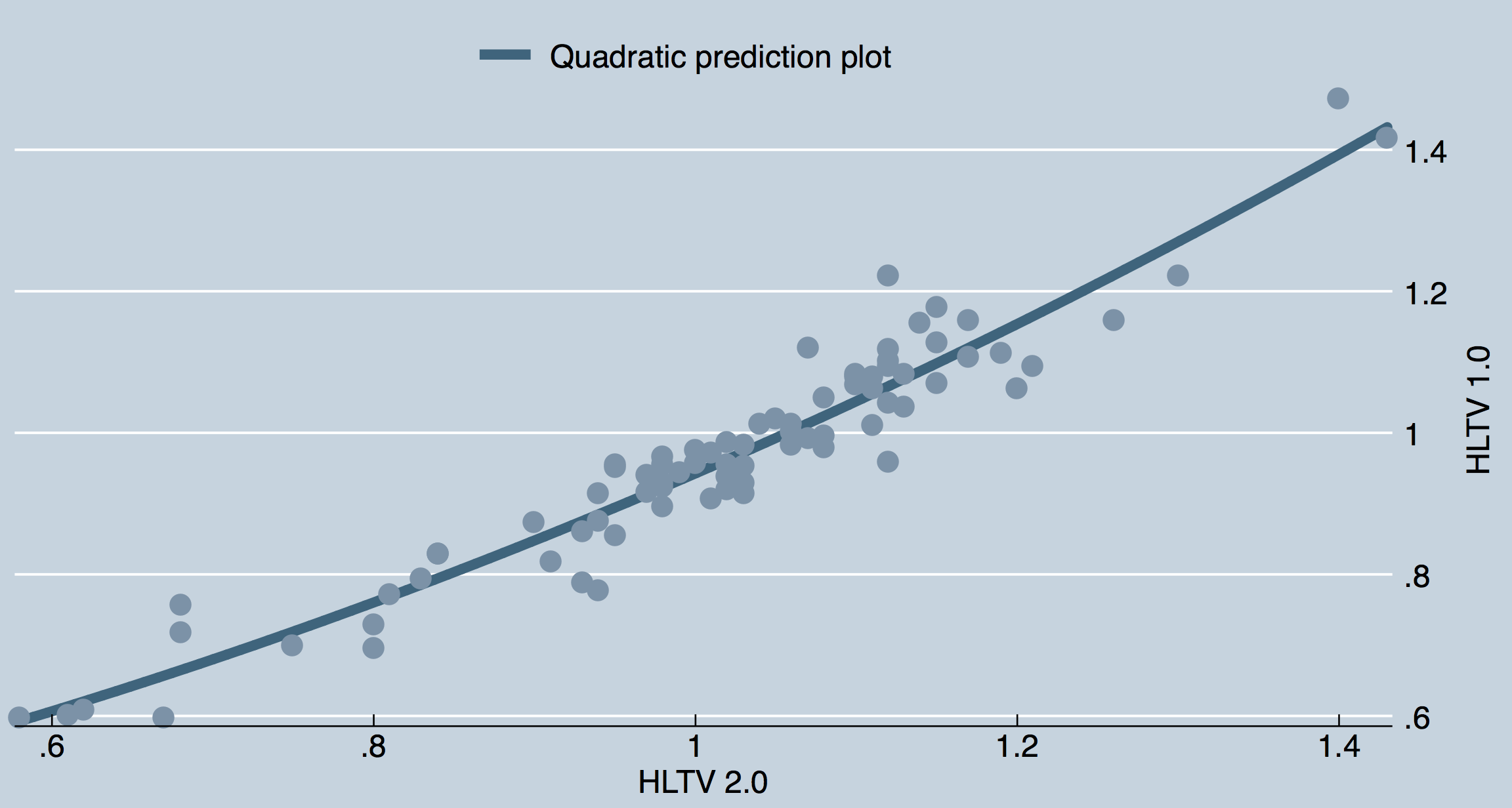
Overall the ratings are quite similar. In fact, their pairwise correlation value is 0.9529. Unsurprisingly, the two rating systems are highly correlated.
HLTV decided against releasing the formula for rating 2.0, but this does not mean we cannot use the same type of econometric analysis to predict something very close using the same variables. Using this method we can also compare this new system to the older system by determining how the variables that affected rating 1.0 affect 2.0.
As with rating 1.0, there are identical problems with what variables influence the outcome the most.
To test this variable using the 200,000+ observations in the HLTV dataset, we must first generate the K/D variable.
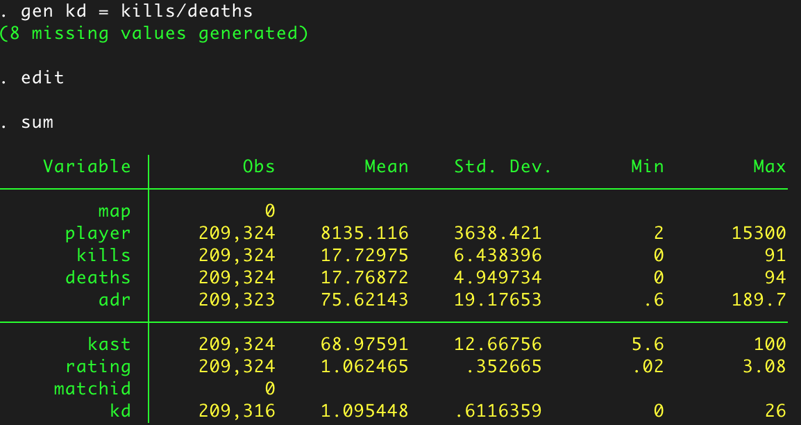
This also gives us some interesting information about aggregated player performance: the average player has a KAST ratio of 69% while the mean rating is 1.06, slightly larger than the target average rating of 1.0.
Now that we have the variable we can run the simple regression:
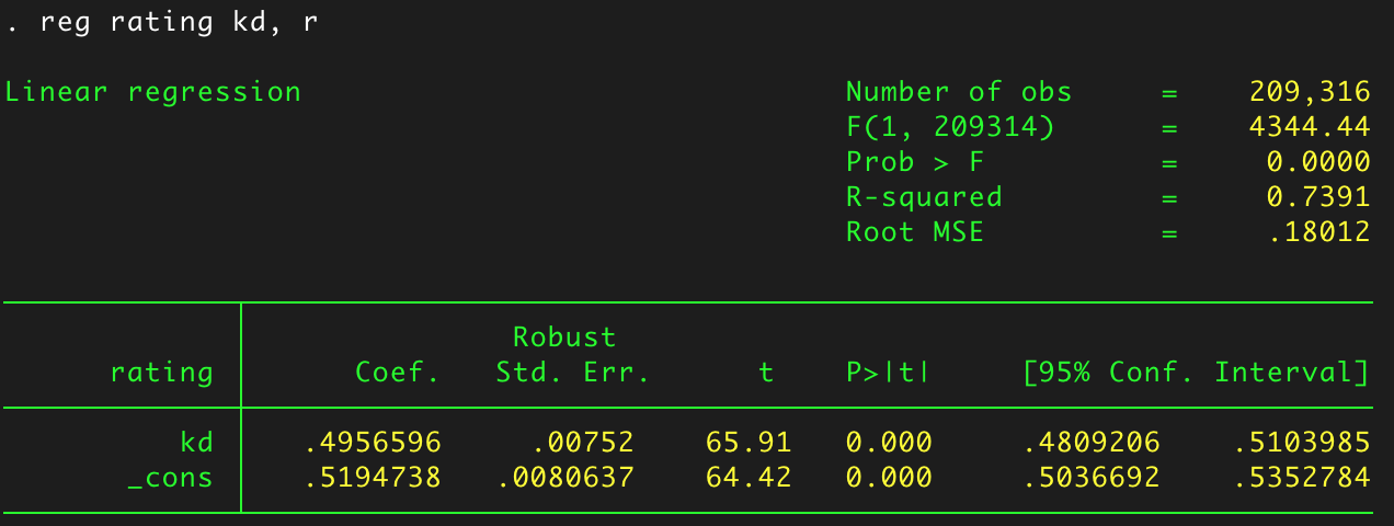
This tells us that KD alone explains 74% of the change in Rating 2.0. While this is down from the 88% of rating 1.0, it does not demonstrate a remarkable shift from the reliance on K/D as a metric for determining player performance.
In fact, when testing separately on Kills and Deaths in lieu of using their ratio, the R² increases back to 88%:
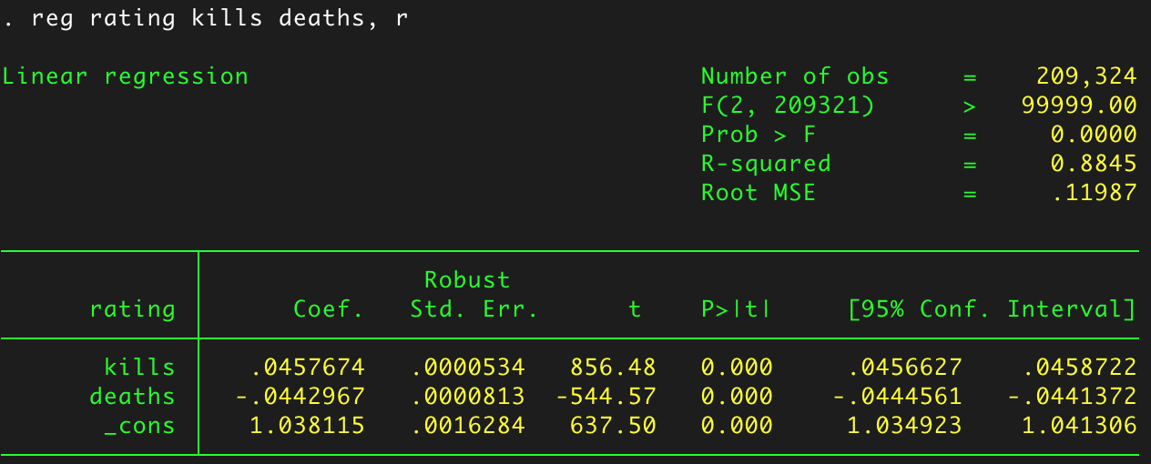
This means that HLTV 2.0’s reliance does not fall squarely on the K/D ratio per-se. However, it is strongly positively correlated with the number of kills a player gets and strongly negatively correlated with the number of deaths a player has.
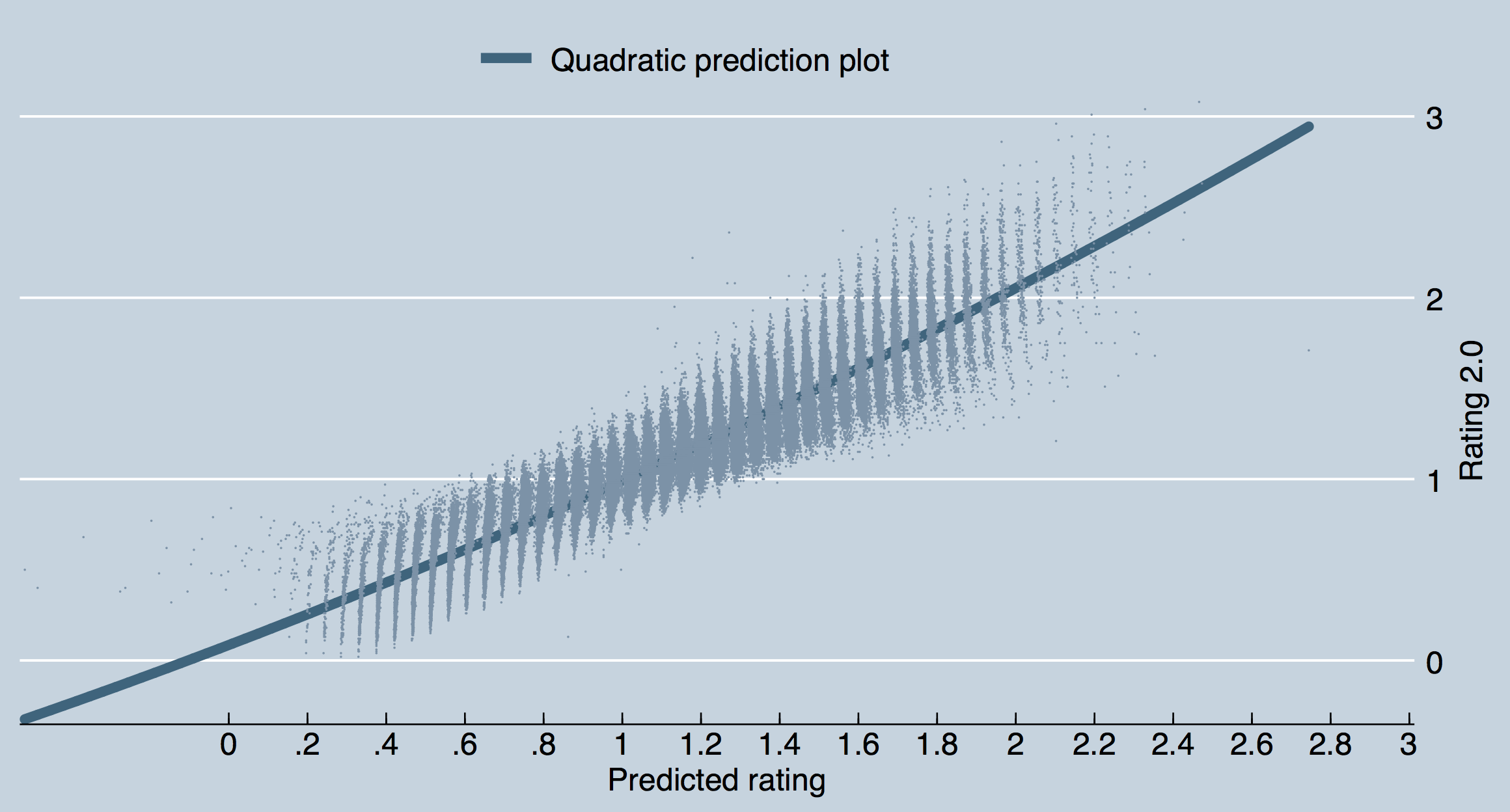
When using this regression equation to predict the value of Rating 2.0 using only Kills and Deaths we see the following trend:
However, with the additional data in the HLTV database, we can increase the accuracy of this prediction.
As established with Rating 1.0, ADR and KAST ratio are significant variables that influence rating. Including them in the earlier regression increases the R² to 95%:
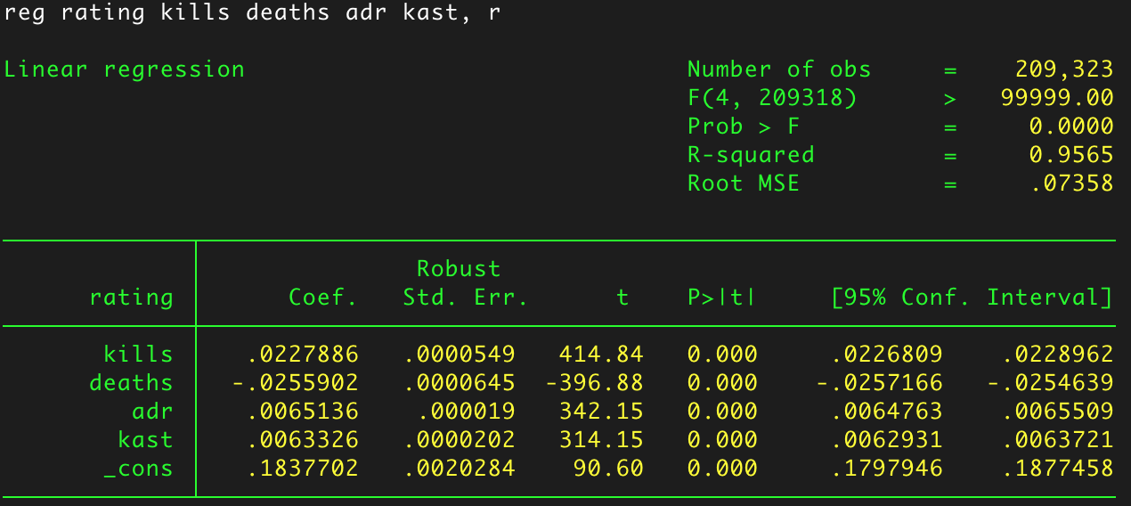
This regression demonstrates that all variables are statistically significant in influencing the value for Rating 2.0. It also evinces that all variables are positively correlated with Rating 2.0 aside from deaths, as we expect. This is different from Rating 1.0 which has a marginal negative correlation to the KAST ratio.
Thus, we can use this formula to predict the value:

Using the above formula we can plot the predicted rating against the actual rating. This correlation is far stronger at 95% R² and lacks the binning pattern in the original rating 2.0 prediction:
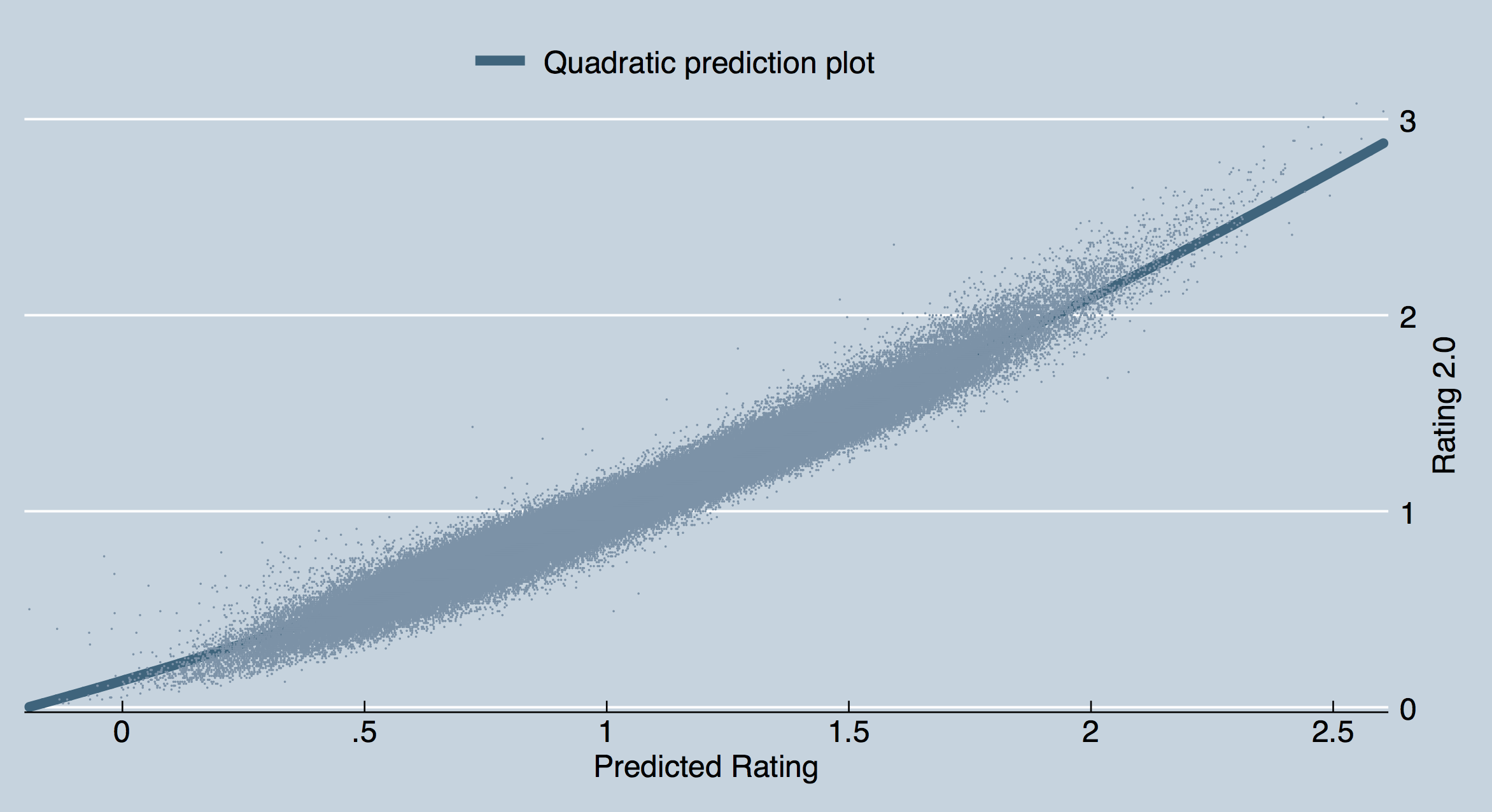
These regressions demonstrate that rating 2.0 simply plots the K/D ratio with little else thrown in to change the number. This does not mean that HLTVs claims that they use ten different pieces of information to calculate the new rating system. However, it does mean that we can arrive at the same conclusion with fewer, less complicated variables.
As a result, we should take rating 1.0 and 2.0 with a grain of salt. The other four statistics that HLTV has on their page are far more telling about different aspects of player performance than these rating systems. Additionally, trade ratios should be accounted for.4
Trade ratios are particularly important as they are not only a measure of team play but also a measure of individual skill: should a player have a high ADR or K/D and low trade death ratio, the numbers evince that player’s aggression has paid off. Likewise, low traded deaths and low K/D would reveal that the same aggression is not paying off. Additionally, entry kills and holds are important factors for determining whether teams can hold a site or enter a site.
As with baseball, it does not make sense to compare pitchers to batters. Similarly, it is not logical to compare riflers, AWPers, entry fraggers, and IGLs. There are ways to measure each of these things distinctly—and we should do so.
Discussion: r/GlobalOffensive